Introduction.
CNN의 Layer는 이미지에서 Feature를 뽑아낸다.
CNN의 출력은 Feature Map으로 표현되고, 더 높은 Layer로 갈수록 Feature들이 Hierarchy하게 쌓이면서 좋은 Feature가 나온다.
최종 Feature는 Classifier 등에서 이용될 수 있다.
그렇다면 아래 논문처럼 CNN에서 Feature Map을 이용하여 이미지를 복원하는 것도 가능할 것이다.
Understanding Deep Image Representations by Inverting Them
그리고 Texture를 분석하고 복원하는 내용을 다룬 논문도 존재한다.
아래 논문은 A Neural Algorithm of Artistic Style 연구팀의 3개월 전 논문이다.
Texture Synthesis Using Convolutional Neural Networks
2015년 발표된 이 논문은 앞선 내용을 바탕으로 CNN에서 Style과 Content를 복원하여 새로운 이미지를 만드는 것을 다룬다.
A Neural Algorithm of Artistic Style
Figure 1.

- Content Reconstructions → Target Image.
- CNN의 처리 단계마다 입력 이미지를 재구성하여 시각화한다.
- 하나의 Higher Layers만을 사용한다.
- a, b, c 같은 Lower Layers에서는 모든 Content가 남아있어 완벽한 복원을 보인다.
-
d, e 같은 Higher Layers에서는 Detailed Pixel Information이 사라지지만, 윤곽 같은 High-level Content는 남아있다.
-
Layers.
conv1_1 (a)- conv2_1 (b)- conv3_1 (c)- conv4_1 (d)- conv5_1 (e)From VGG19 Network.
- Style Reconstructions → Artworks.
- Style Reconstructions를 위해 CNN Representations 위에 Feature Space를 구축했다.
- Style은 같은 Layer의 다른 Features Map 사이의 Correlation으로 정의된다.
- 여러 Layer를 포함하는 Multi-scale이다.
-
Lower Layer에서는 ‘원본 Content’ 정보는 대부분 무시하고 Texture만 복원한다.
복원이 잘 이루어지므로 Correlation이 높다.
-
Higher Layer에서는 ‘원본 Content’ 정보를 포함하여 미술 작품과 비슷한 이미지가 나온다.
복원이 잘 이루어지지 않으므로 Correlation이 낮다.
-
Layers.
conv1_1 (a)- conv1_1, conv2_1 (b)- conv1_1, conv2_1, conv3_1 (c)- conv1_1, conv2_1, conv3_1, conv4_1 (d)- conv1_1, conv2_1, conv3_1, conv4_1, conv5_1 (e)
-
Content Representations와 Style Representations는 분리할 수 있다.
같은 Network를 사용하여 Content와 Style을 복원하고, 그 둘로 새로운 의미 있는 이미지를 만들 수 있다.
Figure 2.

- A: Neckarfront in Tübingen, Germany.
- B: The Shipwreck of the Minotaur by J.M.W. 5 Turner, 1805.
- C: The Starry Night by Vincent van Gogh, 1889.
- D: Der Schrei by Edvard Munch, 1893.
- E: Femme nue assise by Pablo Picasso, 1910.
- F: Composition VII by Wassily Kandinsky, 1913.
Figure 3.

열은 CNN Layer에 따른 이미지 생성 결과이고, 행은 Style & Content의 가중치 별 이미지 생성 결과이다.
- CNN Layer가 깊을수록 Style의 특성이 잘 나타난다.
- 행의 숫자는 Content $\alpha$ / Style $\beta$로, 숫자가 클수록 Content의 특성이 잘 나타난다.
- 따라서 우측 하단의 이미지가 가장 Style과 Content가 잘 반영되어 있다.
Methods.
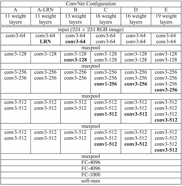
논문에서 CNN Base Network로 VGG19를 사용한다.
VGG19의 구조를 모두 사용하지는 않고, 16개의 Conv Layer와 5개의 Pooling Layer를 사용한다.
Pooling Layer는 Image Reconstruction이라는 목적에 맞게, 기존의 Max Pooling이 아닌 Average Pooling을 사용한다.
-
번외. Average Pooling.

[Part Ⅵ. CNN 핵심 요소 기술] 3. Stochastic Pooling - 라온피플 머신러닝 아카데미 -
Average Pooling은 윈도우 영역에서 평균값을 취하는 방식이다.
VGG의 자세한 내용은 아래 논문을 참고하자.
Very Deep Convolutional Networks for Large-Scale Image Recognition
Content Loss Function.
\[\mathcal{L}_{content}(\vec{p}, \vec{x}, l) = \frac{1}{2} \sum_{i,j} (F^l_{ij} - P^l_{ij})^2. \\ F^l \in R^{N_l \times M_l}\]$x$: Input Image. White Noise.
$p$: Content Image.
$l$: Layer.
$i,j$: $i$ 번째 필터, $j$ 번째 위치.
$F$: $x$를 통과시킨 Feature Map Matrix.
$P$: $p$를 통과시킨 Feature Map Matrix.
Image는 Filter를 통과하면 Encoding 된다.
-
번외. Frobenius Norm.
-
번외. Mean Squared Error(MSE) & Mean Squared Deviation(Difference)(MSD).
블루래더 - 경제적 자유를 향한 푸른 사다리 : 네이버 블로그
\[\frac{\delta \mathcal{L}_{content}}{\delta F^l_{ij}} = \begin{cases} (F^l-P^l)_{ij} \ \text{if} \ F^l_{ij} > 0 \\ 0 \qquad \qquad \ \ \text{if} \ F^l_{ij} < 0. \end{cases}\]
$x$와 $p$의 Content가 얼마나 다른지 나타내는 Loss Function을 최소화하는 값을 찾는다.
해당 식은 Loss를 Layer의 Activations로 미분한 것이다.
Standard Error Back-propagation을 통해 $x$의 Gradient를 계산한다.
그리고 Initially Random Image $x$를 계속 Update한다.
Style Loss Function.
\[G^l_{ij} = \sum_k F^l_{ik}F^l_{jk} \qquad (G^l \in R^{N_l \times N_l}). \\ E_l = \frac{1}{4N^2_lM^2_l} \sum_{i,j} (G^l_{ij} - A^l_{ij})^2 \\ \mathcal{L}_{style}(\vec{a}, \vec{x}) = \sum^L_{l=0} w_l E_l\]$x$: Input Image. White Noise.
$a$: Style Image.
$G$: Gram Matrix.
$A$: $a$를 통과시킨 Feature Map Matrix.
$E$: Style Loss Contribution.
$i,j$: $i$ Feature Map, $j$ Feature Map.
$N_l$: $l$ Layer의 Filter 개수.
$M_l$: $l$ Layer에서 Filter의 가로 세로 곱.
-
Gram Matrix.
Style은 같은 Layer의 다른 Features Map 사이의 Correlation이고, Filter의 개수는 $N_l$이므로, $R^{N_l \times N_l}$이다.
$l$ Layer에서, $i$ Feature Map과 $j$ Feature Map을 내적하여 Correlation을 구한다.
이렇게 계산하여 나온 Matrix가 Gram Matrix이다.
Expectation에 대한 내용은 인용문을 참고하자.
이때, correlation을 계산하기 위하여 각각의 filter의 expectation 값을 사용하여 correlation matrix를 계산한다고 한다. 즉, l번째 layer에서 필터가 100개 있고, 각 필터별로 output이 400개 있다면, 각각의 100개의 필터마다 400개의 output들을 평균내어 값을 100개 뽑아내고, 그 100개의 값들의 correlation을 계산했다는 것이다.
-
Style Loss Contribution & Style Loss.
$L$은 Loss에 영향을 주는 Layer 개수이다.
$w_l$은 활성화할 Layer를 나타내는 가중치로, 합은 1이다.
선택한 레이어를 제외하고 모두 0으로 만드는 방법을 사용한다.
e.g. Figure 3의 a 그림은 conv1_1만 선택되므로 conv1_1의 $w_l=1$이고, 나머지는 0이다.
\[\frac{\delta E_l}{\delta F^l_{ij}} = \begin{cases} \frac{1}{N^2_l M^2_l} ((F^l)^T (G^l - A^l))_{ji} \ \text{if} \ F^l_{ij} > 0 \\ 0 \qquad \qquad \qquad \qquad \qquad \text{if} \ F^l_{ij} < 0. \end{cases}\]
$x$와 $a$의 Style이 얼마나 다른지 나타내는 Loss Function을 최소화하는 값을 찾는다.
해당 식은 Loss를 Layer의 Activations로 미분한 것이다.
Standard Error Back-propagation을 통해 $x$의 Gradient를 계산한다.
Total Loss Function.
\[\mathcal{L}_{total}(\vec{p}, \vec{a}, \vec{x}) = \alpha \mathcal{L}_{content}(\vec{p}, \vec{x}) + \beta \mathcal{L}_{style}(\vec{a}, \vec{x})\]Content Loss와 Style Loss의 합을 최소화한 값이다.
$\alpha$와 $\beta$는 Figure 3에서 행의 값을 정하는 요소이다.
보통 $\alpha/\beta = 10^{-3}, \, 10^{-4}$을 사용한다.
링크.
고흐의 그림을 따라그리는 Neural Network, A Neural Algorithm of Artistic Style (2015) - README